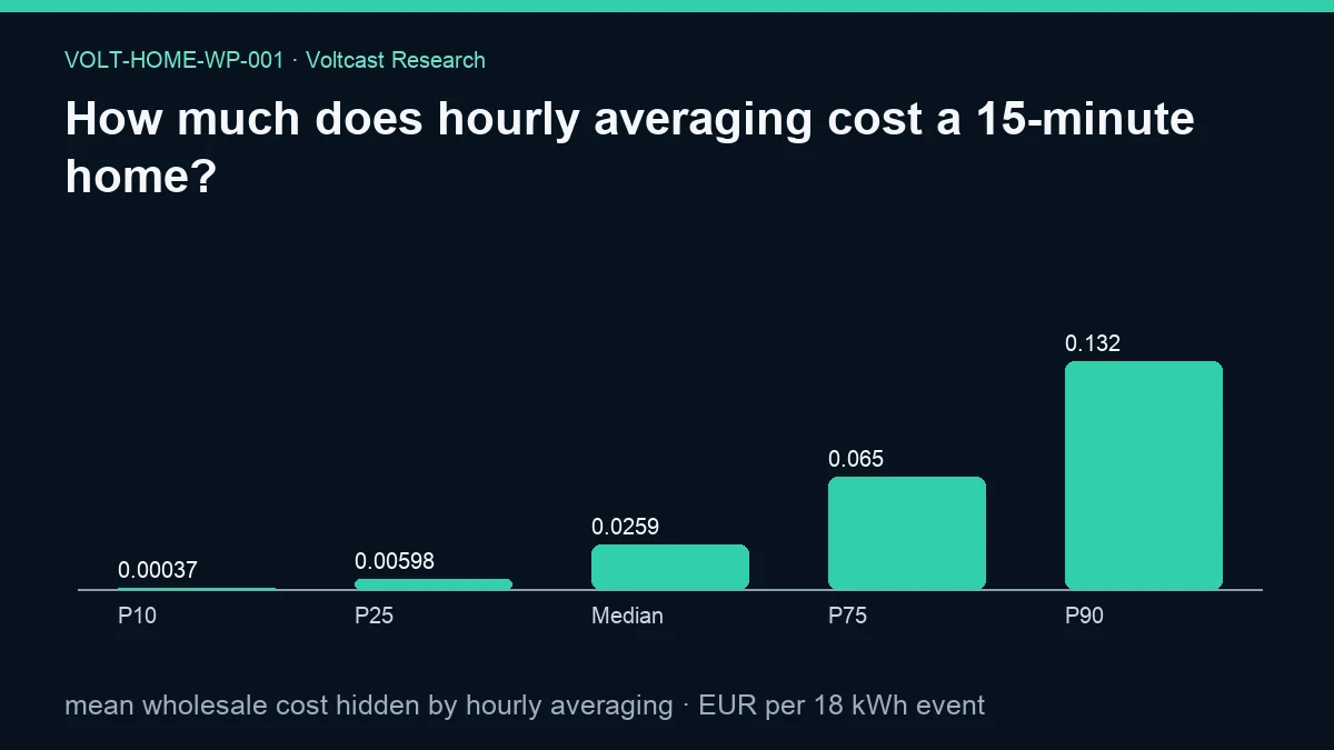
How much does hourly averaging cost a 15-minute home?

Abstract

Electricity delivered in quarter-hour intervals can contain price variation that disappears when those intervals are represented by one hourly average. This working paper measures the consequence for a stylized flexible household event. Using complete native-resolution delivery curves, it compares a schedule selected from quarter-hour prices with a schedule exposed to hourly averaging. The recorded primary result is a mean hidden wholesale cost of €0.051148916066066016 per 18 kWh event across 3,330 observations, with a day/row-block mean-bootstrap interval from €0.04632943354861107 to €0.05265177113263883. Positive values mean that the native quarter-hour selection found a cheaper schedule.

The result is deliberately narrow. It uses an assumed 18 kWh event, an assumed 7.4 kW charger, perfect day-ahead foresight, and wholesale energy prices only. Taxes, supplier margin, and network charges are excluded. It is therefore neither an estimate of a household bill nor evidence about realized customer savings. The analysis and drafting were model-assisted. This paper is not peer reviewed and is not trading advice.

Plain-language answer

Hourly averaging hid a small but measurable amount of wholesale scheduling value in this reconstruction. The measured mean was about five euro cents for the assumed 18 kWh event. That is the difference between two representations of the same delivery curve, not a promise that a household will save that amount. A retail bill combines wholesale energy with taxes, network charges, supplier terms, device losses, and constraints that this paper does not model.

The practical lesson is about information fidelity. If a market and device can act at quarter-hour resolution, replacing four distinct quarter-hour prices with one average can erase the order of cheap and expensive intervals inside the hour. An optimizer can then choose an hour correctly while still choosing the wrong parts of that hour. Conversely, a household whose tariff, meter, or device is genuinely settled and controlled only hourly may not be able to realize the measured difference. Native data is useful only when the rest of the control chain preserves it.

The magnitude should also be read in context. The study assumes perfect foresight of the day-ahead curve. It does not test forecast error, late device arrival, a changing energy requirement, failed commands, battery degradation, or comfort. The answer is consequently: hourly averaging can cost schedule quality, and the corpus detects that cost, but the result is a wholesale-resolution diagnostic rather than a household savings study.

Research question

The research question is whether converting native quarter-hour day-ahead prices into hourly averages changes the cost of a flexible household schedule. More precisely, the estimand is the paired wholesale-cost difference between selection on the native curve and selection after hourly aggregation for the assumed event.

This framing separates a data-resolution question from broader tariff economics. It does not ask whether a dynamic tariff is better than a fixed tariff, whether a charger owner recovers hardware costs, or whether all homes should automate. It asks what information is lost before those downstream questions are considered. A positive paired difference supports the limited claim that native quarter-hour ordering can expose cheaper intervals that an hourly average conceals.

Data and provenance

The evidence artifact identifies three data windows. Daily prices cover 2021-01-01 through 2026-08-29. Detailed intervals cover 2025-10-01 through 2026-08-29. The longer historical window covers 2015-01-01 through 2026-08-29. The detailed interval limitation is material: the interval analysis uses ten representative European bidding zones beginning on 2025-10-01. The paper does not generalize that sample to every European zone or every historical market regime.

The source contract names the zones, day_ahead_prices, grid_revisions, auction_publications, and ingestion_runs tables. The analysis ran in a read-only transaction with a statement timeout of 180 seconds and a publication cutoff of 2026-08-30T00:00:00Z. The frozen production snapshot is identified by SHA-256 7e97489fc8528c8cc8c38830e05b48d949ce1f67b98575dff26f5d7c321e4c67. The analysis-code hash is 57c57de79cdab2b5b6d6c54c485cb5162598c5ba0b0bfe995da40d75e6c52ba9, the protocol hash is adb36bf6b447af9f96339249b8becaefc20422499cca1977242866347a97bd4b, the paper-registry hash is 7bcb91d7476d0a69fe9fa75a5c7782f8117e0153f82f9112b7e1d307d3943717, and the source-registry hash is 07949550ac443ff673fda5c0209b99f137544f3ffecf6775f109bb9d09663bd6. The evidence manifest records evidence SHA-256 d04e8d7e38e69e5d00b5634e84e4d4c978d7d7391c02deb819dc9b146a9641f5 and figure SHA-256 4cc9925f9b24e351d6343a45223d56dcfe1c24c99a584c2d1e4b4a24e62757ee.

These hashes establish identity, not correctness by themselves. They allow a reviewer with access to the canonical materials to verify that the public aggregate points to the frozen inputs, protocol, registry, and implementation. Licensing and redistribution conditions are handled separately through the stated licensing route; this public paper reports paper-level aggregates rather than reproducing the underlying market payload.

Method

The method belongs to the registered family of paired interval reconstruction, clock-safe counterfactuals, and day-block bootstrap. For each eligible event, the native quarter-hour curve is retained as the decision surface. A corresponding hourly representation is formed by averaging the prices inside each hour. Schedules are then compared on a paired basis so that both representations refer to the same underlying delivery day and event assumptions.

The event is synthetic. Its energy requirement is fixed at 18 kWh and its charger power at 7.4 kW. Perfect day-ahead foresight is assumed, so the schedule uses realized day-ahead prices rather than a forecast available under uncertainty. This is an upper-fidelity comparison of interval representations, not a prospective controller test. The cost includes wholesale energy only. Taxes, network charges, supplier margin, and any fixed retail components are outside the estimand.

Pairing matters because price levels differ across zones and days. Comparing native schedules from one set of days with hourly schedules from another would mix the effect of resolution with market conditions. Here, the difference is computed within the same eligible event. The primary metric is the mean wholesale cost hidden by hourly averaging, expressed in euros per assumed event.

The artifact labels the interval method day/row-block mean bootstrap, rather than treating every interval as independent. That choice retains the registered block structure instead of substituting an interval-level resample. The evidence registers within-family Holm control for inferential claims, while classifying this result as descriptive and making no unadjusted significance claim.

Results

Across 3,330 paired events, the recorded mean wholesale cost hidden by hourly averaging is €0.051148916066066016 per 18 kWh event. The day/row-block mean-bootstrap interval runs from €0.04632943354861107 to €0.05265177113263883. The interval remains positive, matching the evidence interpretation that native quarter-hour selection found a cheaper schedule than the hourly representation.

The figure shows the event-level distribution at P10, P25, median, P75, and P90. In that order, the plotted values are €0.0003698499999999895, €0.005978874999999884, €0.02586880555555554, €0.06498558333333315, and €0.1322851 per event. Those quantiles describe dispersion and are distinct from the primary mean and its interval.

This is a resolution effect measured under the study assumptions. It does not mean each event incurs the mean, and it does not convert directly into an annual amount. The evidence artifact does not report an annual event count, a household participation rate, or a retail pass-through rule, so this paper does not manufacture those quantities. It also does not claim that averaging changes the physical market price. Averaging changes what the optimizer can see and therefore can change the selected delivery intervals.

The finding is economically modest at the single-event level but technically clear: preserving native granularity retains information that aggregation discards. Whether that information is valuable to a particular household depends on tariff settlement, device controllability, and the costs omitted here.

Robustness and placebo checks

The paired design is the principal control. Native and averaged schedules are reconstructed from the same event and delivery curve, limiting contamination by day-level price regimes or zone-level price differences. Clock-safe handling is part of the registered method family, which is important because quarter-hour grouping can otherwise be corrupted at local-time boundaries.

The recorded day/row-block mean bootstrap is the reported robustness measure. Its interval follows the block implementation named in the evidence rather than an independent-interval calculation. The result is not presented as an unadjusted discovery among many papers. Within-family Holm control governs inferential claims, and this paper remains descriptive.

Several useful checks are boundaries rather than additional measurements. Perfect foresight means no forecast placebo was run here. Wholesale-only costing means no retail-tariff placebo was inferred. The paper also does not substitute an hourly device for a quarter-hour device and call that a validation. Those would answer different questions. The strongest internal comparison is the matched representation change while holding the synthetic event and observed curve fixed.

Limitations

The detailed analysis covers ten representative European bidding zones from 2025-10-01 through 2026-08-29. Representation does not imply complete European coverage. Market design, liquidity, tariff pass-through, and native settlement differ, so the mean should not be transported to an unobserved zone without a corresponding measurement.

The 18 kWh requirement and 7.4 kW charger are assumptions, not observations about the household population. Perfect foresight is also an assumption. Real automation makes decisions with publication delays, forecast uncertainty, changing availability, and device or communication failures. Any of these may reduce, erase, or occasionally change the sign of realized value.

Only wholesale energy is priced. Taxes, supplier margin, and network charges are excluded, as are charging losses, equipment costs, battery wear, demand charges, and behavioral constraints. For that reason, this is explicitly not a household bill study. It cannot establish payback, adoption value, or consumer welfare.

Finally, a positive mean is not a universal guarantee. The public evidence reports the aggregate primary metric and bootstrap interval, not a claim that every underlying event benefited. The paper therefore avoids individual-day promises and annual extrapolation.

Practical implication

Home-energy software should preserve native market intervals from ingestion through scheduling whenever the tariff and device can use them. That means retaining interval start and end times, zone identity, resolution, and timezone semantics rather than flattening the curve into hourly labels too early. Aggregation can still be offered for display or for genuinely hourly devices, but it should be an explicit transformation rather than the canonical record.

A safe controller should also test the whole chain. Native data offers no benefit if an integration rounds timestamps, a tariff bills hourly, or a charger accepts only coarser commands. Product claims should describe that boundary. The measured result supports “resolution can affect wholesale schedule selection,” not “quarter-hour automation will lower every bill.”

For a household, the appropriate decision is operational rather than speculative: verify the tariff's settlement interval, the meter's data interval, and the device's command interval. If all preserve quarter-hour control, native prices contain information worth retaining. If one link collapses the signal, the optimizer should represent that constraint honestly instead of reporting synthetic precision.

Reproducibility

The public evidence JSON at /research-data/home-papers/how-much-does-hourly-averaging-cost-a-15-minute-home.json is the machine-readable reproduction entry point. It provides the title, status, assumptions, windows, source tables, primary metric, sample size, unit, bootstrap interval, limitations, disclosure, and provenance hashes. The accompanying figure is identified in frontmatter and carries alternative text copied from that artifact.

A reproduction should verify the protocol, paper-registry, source-registry, snapshot, analysis-code, evidence, and figure hashes before recomputing. It should use the stated publication cutoff, preserve the read-only transaction boundary, reconstruct complete native delivery intervals with clock-safe timestamps, form hourly averages deterministically, and compare paired schedules for the same assumed event. Interval recomputation should follow the recorded day/row-block mean-bootstrap implementation. A differing result should not be reconciled by silently changing the event, zones, cutoff, interval completeness rule, or price source.

The source registry is also part of interpretation. The official market-coupling materials describe the day-ahead context and product framework, while the architecture document describes the system boundary. The Google policy source is included because public model-assisted work must add original evidence rather than scaled paraphrase. None of those sources replaces the measured JSON; they establish context around the frozen aggregate.

Disclosure

Analysis and drafting were model-assisted; sources, code, assumptions, and evidence hashes are disclosed. This public working paper is not peer reviewed. It is not a household bill study and is not trading advice. Volt has zero live traders and zero live trading capital; C0R is the only paper strategy. Production weather forecasting is a non-trading service. No live order, capital authorization, or trading claim follows from this household-resolution analysis.

References

• Spam Policies for Google Web Search — Scaled content abuse — Google Search Central.
• Single Day-ahead Coupling (SDAC) — ENTSO-E.
• EU electricity trading in the day-ahead markets becomes more dynamic — European Commission.
• ACER Decision 13-2024 on SDAC Products — Agency for the Cooperation of Energy Regulators.
• Voltcast Architecture — Voltcast.