How taxes and network charges dilute the wholesale price signal
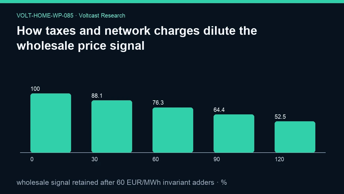
How taxes and network charges dilute the wholesale price signal. Invariant taxes do not change interval rank, while time-varying network charges can; this scenario shows magnitude dilution.
Abstract
Taxes, network charges, and supplier components can make wholesale electricity variation a smaller part of the total price a household sees. This working paper measures that dilution through a deliberately simple signal-to-adder sensitivity. It starts with the mean daily maximum-minus-minimum wholesale price range and asks what percentage remains after subtracting an illustrative invariant adder of €60/MWh, floored at zero, then dividing by the original mean range. Across 93,161 observations, the registered result is 76.2665240334153%. The €60/MWh input is a declared synthetic wholesale scenario assumption, not a quoted tax, network tariff, or retail charge for any country. A constant adder applied equally to every interval would not alter interval ordering or the mathematical maximum-minus-minimum spread. The registered percentage instead measures the adder’s magnitude relative to the average wholesale range. Time-varying network charges could change the preferred interval, but that case is not computed here. The analysis uses no customer bills or telemetry and makes no customer-saving claim.
Plain-language answer
The frozen sensitivity reports that 76.2665% of the mean wholesale-range signal remains after the formula subtracts an illustrative €60/MWh adder. This does not mean a household retains 76.2665% of its savings. There are no measured savings in the analysis, and the €60/MWh input is not a real tariff quote.
It is also important to separate two effects. If exactly the same €60/MWh is added to every interval, the cheapest wholesale interval remains the cheapest and the most expensive remains the most expensive. Their difference is unchanged. What changes is how large that difference looks relative to the all-in price level. By contrast, a network charge that is high in one time block and low in another can reorder intervals. A controller following wholesale prices alone might then choose the wrong all-in period.
This paper quantifies only the first kind of salience or magnitude dilution, using a subtractive ratio. It does not simulate the second kind of time-varying tariff conflict. Every euro figure is an illustrative synthetic wholesale scenario, never a customer saving or retail bill. The practical message is to optimize against the complete marginal tariff, not to assume wholesale ordering automatically equals retail ordering.
Research question
The research question asks how non-wholesale charges dilute a wholesale price signal. The implemented estimand is the fraction of the mean observed daily wholesale range left by a specific normalization after a €60/MWh illustrative adder.
It does not estimate a tax incidence, compare national retail tariffs, or identify the causal effect of network pricing. “Retained” refers to a constructed signal ratio, not money retained by a customer. The question also distinguishes invariant and time-varying additions: the former affects price composition but not interval rank; the latter may affect both composition and scheduling.
Data and provenance
The underlying evidence comes from a frozen, SELECT-only production snapshot containing no customer telemetry. Registered source contracts are day_ahead_prices, forecast_accuracy, bess_index_daily, zone_load, and zone_holidays. This paper’s primary computation uses daily maximum and minimum day-ahead prices to form ranges. The evidence reports 93,161 observations.
The daily-price window is 2021-01-01 through 2026-08-29. The registered corpus also contains detailed-interval coverage from 2025-10-01 through 2026-08-29 and a long-history boundary from 2015-01-01 through 2026-08-29. The publication cutoff is 2026-08-30T00:00:00Z. These dates define the frozen corpus; they do not turn the illustrative adder into a historically observed retail component.
The snapshot SHA-256 is 7e97489fc8528c8cc8c38830e05b48d949ce1f67b98575dff26f5d7c321e4c67. The protocol hash is adb36bf6b447af9f96339249b8becaefc20422499cca1977242866347a97bd4b, the paper-registry hash is 7bcb91d7476d0a69fe9fa75a5c7782f8117e0153f82f9112b7e1d307d3943717, the source-registry hash is 07949550ac443ff673fda5c0209b99f137544f3ffecf6775f109bb9d09663bd6, and the analysis-code hash is 57c57de79cdab2b5b6d6c54c485cb5162598c5ba0b0bfe995da40d75e6c52ba9. The evidence-manifest hashes are 34fb9894dfa75990013b5fd1c30dbb333d909d696db730862646b9bf7670f401 for the JSON and 8ccac3421de160d502ed1ddf0d0ee8e1075ba4d53afe7a4f84fb687c37c53884 for the WebP figure. Extraction used a read-only transaction with a 180-second statement timeout. The external references are contextual; the result is bound to the Volt evidence and the declared €60/MWh synthetic input.
Method
For each included zone-day, the analysis computes the wholesale range:
daily maximum day-ahead price - daily minimum day-ahead price.
It then takes the arithmetic mean of those daily ranges. For each illustrative adder in the figure—€0, €30, €60, €90, and €120 per MWh—the retained percentage is:
100 × max(mean daily range - adder, 0) ÷ mean daily range.
The registered primary scenario selects the €60/MWh case. This is a sensitivity index. It is not the result of adding €60/MWh to every interval and recomputing the interval range; doing that would leave the range unchanged. The index instead compares the size of an adder with the size of the average daily wholesale spread.
The evidence assumptions describe a 4,000 kWh annual synthetic household, a 35% flexible-energy share, wholesale pass-through, no customer telemetry, and illustrative invariant adders. Annual load and flexible share do not enter the retained-percentage formula. Consequently, the result is not an annual monetary amount.
No country’s taxes or network schedule is loaded. VAT, supplier margin, fixed fees, and device losses are excluded. No EV, battery, or heat pump is simulated. Battery round-trip efficiency and degradation, EV charging losses and availability, and heat-pump COP and comfort therefore remain unmodeled rather than assumed away. Any monetary value discussed is a declared synthetic wholesale scenario.
Results
The registered primary result is 76.2665240334153%. Rounded, the formula retains 76.27% of the mean wholesale-range signal after the illustrative €60/MWh subtraction. The sample size is 93,161 price observations.
This percentage describes relative magnitude under the formula. It does not measure customer savings, bill pass-through, tax burden, or network-cost avoidance. It also does not imply that the remaining wholesale signal changes which interval is cheapest. Under a truly invariant adder, interval ranking stays the same.
The supplied interpretation explicitly distinguishes these points: invariant taxes do not change interval rank, while time-varying network charges can; the scenario shows magnitude dilution. The measured percentage supports only the declared magnitude comparison. No time-varying charge series is present, so no frequency of ranking reversals can be reported.
The figure values are exactly 100.0%, 88.13326201670765%, 76.2665240334153%, 64.39978605012294%, and 52.53304806683059% at illustrative adders of €0, €30, €60, €90, and €120/MWh. The regenerated evidence reports bootstrap_95_interval: null and interval_method: "not reported for this estimand", so no uncertainty interval is claimed.
Robustness and placebo checks
The frozen figure provides a deterministic adder grid from €0 to €120/MWh. At €0/MWh, the retained index must be 100%. As the illustrative adder rises, the index declines linearly until the floor binds at zero. This verifies the formula’s monotonic behavior but does not show how any country’s tariff behaves.
An invariant-adder placebo should apply the same amount directly to every interval before calculating the daily range. The recomputed maximum-minus-minimum spread must equal the original spread, apart from numerical precision. This placebo demonstrates that the primary index measures salience relative to an adder, not loss of arbitrage spread caused by a constant fee.
A time-varying robustness study would use a registered network schedule, combine it with wholesale prices interval by interval, and count how often the all-in cheapest period differs from the wholesale cheapest period. It would preserve local time, daylight-saving transitions, weekends, seasons, and jurisdiction. That test is necessary for scheduling claims but is outside this evidence.
A household-load robustness study would weight prices by a declared standardized profile and compare full synthetic cost under wholesale-only and all-in schedules. The current 4,000 kWh and 35% assumptions do not perform that weighting. No annual euro result is inferred here.
The tariff family applies Holm correction to inferential claims and requires blocked day or week bootstrap intervals for serial dependence. This paper reports a descriptive sensitivity and makes no significance claim.
Limitations
The €60/MWh adder is illustrative. It is not metadata about a country, retailer, tax year, or network operator. The €0–€120/MWh grid is likewise a scenario grid, not a survey of actual tariffs. Treating it as current retail data would invent findings absent from the source registry and evidence.
The primary formula subtracts an invariant adder from a spread even though directly adding a constant to interval prices leaves that spread unchanged. The output is therefore best understood as a normalized signal-salience index. It is not a physical or accounting decomposition of an electricity bill.
Time-varying charges, which can alter interval rankings, are not modeled. Neither are VAT interactions, supplier markups, fixed monthly fees, price caps, rebates, balancing adjustments, or negative-price pass-through rules. The study cannot tell a household which period is cheapest on its complete tariff.
Annual consumption and flexible share are declared but not used in the primary percentage. No load shape or asset schedule appears. There are no efficiency, degradation, power, state-of-charge, comfort, or availability assumptions because devices are not modeled. Historical wholesale dispersion is pooled across the snapshot and may not describe one zone or future period.
Finally, the evidence reports no interval for the primary metric. The result is descriptive and deterministic given the frozen mean range and selected adder.
Practical implication
Home-energy optimization should use the full marginal price for each interval. Constant charges may matter greatly for total affordability while leaving the preferred interval unchanged. Time-varying taxes or network charges can change both total cost and the scheduling decision.
Use 76.2665% only as the registered signal-to-adder sensitivity for an illustrative €60/MWh input. Do not use it as a savings-retention rate. A decision-grade extension should load a named tariff, preserve every time rule, add the household’s profile and device constraints, and report synthetic all-in results separately from observed bills.
Reproducibility
Verify the frontmatter evidence record’s stable ID, slug, title, assumptions, status, cutoff, source tables, all five provenance hashes, and the evidence-manifest hashes for the JSON and figure. Confirm that extraction was read-only and that the snapshot hash matches the manifest.
From the frozen daily prices, compute each maximum-minus-minimum range and their arithmetic mean. For the primary scenario, evaluate 100 × max(mean range - 60, 0) / mean range. The output should reproduce 76.2665240334153%. Repeat with adders 0, 30, 60, 90, and 120 EUR/MWh to reproduce the figure.
Do not substitute actual national tariff metadata without registering its source and effective date. Applying a constant directly to every interval, or applying a time-varying schedule, answers a different question and must receive distinct evidence.
Disclosure
Analysis and drafting were model-assisted. This public working paper is not peer reviewed. Its adder is illustrative, its evidence is frozen, and its formula and omissions are disclosed. It is not financial, tariff-selection, investment, purchasing, or trading advice.
Every euro-denominated amount is a declared synthetic wholesale scenario, not a customer saving or retail bill. Volt has no live traders or live capital; C0R is the only paper strategy, and this study is not trading research.
References
- Advances in Applied Energy, Assessing the conditions for economic viability of dynamic electricity retail tariffs for households.
- ACER and CEER, Rewarding flexibility: How retail contract choice can help unlock consumer flexibility.
- European Commission, Communication from the Commission on the Citizens Energy Package.
- Energy Policy, Welfare redistribution through flexibility — Who pays?.
- International Energy Agency, Scaling Up Demand Flexibility.