How much flexibility do 3.7, 7.4, 11, and 22 kW chargers create?

Abstract

Charger power changes how much energy can be concentrated into a low-priced interval. This paper compares optimized wholesale scenario cost for an 18 kWh event at 3.7 kW, 7.4 kW, 11 kW, and 22 kW. The common scenario assumes wholesale energy only, perfect charger efficiency, and local availability from 17:00 to 07:00. Across a sample size of 3,330, the measured wholesale scenario cost difference between 3.7 kW and 22 kW is €0.11122826001100294 per event. Higher power lowers the modeled optimum because the scheduler can place the required energy into fewer of the cheapest intervals, but the result is conditional on recorded curves and excludes vehicle, connection, loss, tariff, and behavioral constraints. The regenerated evidence reports no interval for this estimand, so no confidence interval is claimed for €0.11122826001100294.

Plain-language answer

In this scenario, more charger power creates scheduling flexibility by shortening the time needed to deliver 18 kWh. A 22 kW optimizer can concentrate energy into fewer cheap intervals than a 3.7 kW optimizer. The measured difference is a wholesale scenario value of €0.11122826001100294 per event in favor of the higher-power optimum.

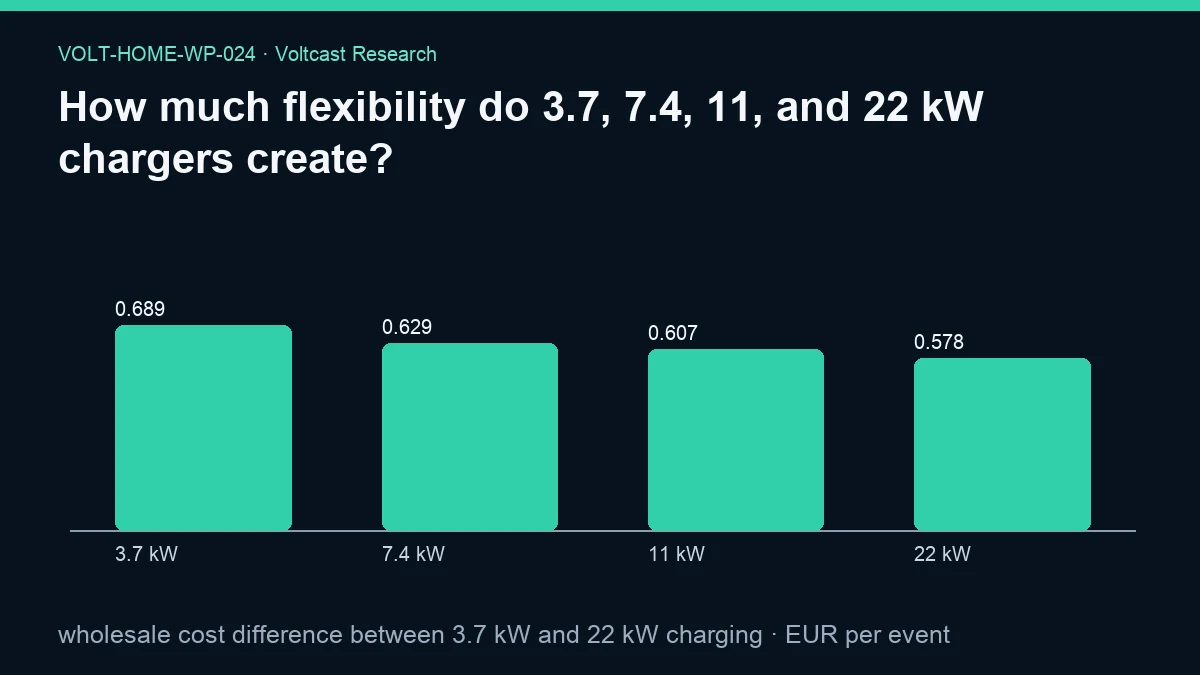
That does not mean a 22 kW installation produces that amount for a driver. A vehicle may accept less power, a connection may limit simultaneous load, and real conversion is not perfectly efficient. It also does not mean power creates cheap prices. Power only changes the feasible response to a price curve. Once enough power is available to fit the event into the best intervals, additional power may have little scheduling value. The figure publishes the four wholesale scenario costs: 3.7 kW = 0.6892939216876496, 7.4 kW = 0.6286570366986219, 11 kW = 0.6072459371257485, and 22 kW = 0.5780656616766466 EUR per event.

Research question

The question is: with energy need and availability held fixed, how does charger power alter the minimum wholesale scenario cost of price-aware EV charging?

The comparison covers 3.7 kW, 7.4 kW, 11 kW, and 22 kW. Every arm must deliver 18 kWh against the same recorded interval prices. Power affects the maximum energy assignable to each interval and therefore the number of intervals needed. This isolates one technical source of flexibility: concentration capacity.

The question is not whether a higher-power charger is economically worthwhile after equipment, connection, or demand charges. Those inputs are absent. It also does not test charging speed as convenience. The estimand is a paired wholesale scenario cost difference under one optimization model.

Data and provenance

The evidence contract names day_ahead_prices, forecasts, forecast_accuracy, generation_mix, and zones. Recorded prices and zone timezones directly support the power comparison. No charger telemetry, vehicle acceptance curve, household load, or installation cost is included.

The declared daily-price window is 2021-01-01 through 2026-08-29; detailed intervals cover 2025-10-01 through 2026-08-29; and long history covers 2015-01-01 through 2026-08-29. The publication cutoff is 2026-08-30T00:00:00Z. Extraction was read-only with a 180-second statement timeout.

The snapshot SHA-256 is 7e97489fc8528c8cc8c38830e05b48d949ce1f67b98575dff26f5d7c321e4c67. Protocol, registry, source-registry, and analysis-code hashes are adb36bf6b447af9f96339249b8becaefc20422499cca1977242866347a97bd4b, 7bcb91d7476d0a69fe9fa75a5c7782f8117e0153f82f9112b7e1d307d3943717, 07949550ac443ff673fda5c0209b99f137544f3ffecf6775f109bb9d09663bd6, and 57c57de79cdab2b5b6d6c54c485cb5162598c5ba0b0bfe995da40d75e6c52ba9. These frozen identities are the provenance boundary for every empirical claim.

Method

For each eligible zone-day, recorded intervals are ordered by day-ahead price. The scheduler allocates an 18 kWh requirement from cheapest upward. In each interval, deliverable energy is limited by charger power multiplied by recorded interval duration. Allocation stops when the requirement is met; an incomplete final interval may supply only the remaining energy.

The calculation is repeated at 3.7 kW, 7.4 kW, 11 kW, and 22 kW. Perfect efficiency means input energy and delivered energy are treated as equal. Wholesale scenario cost is interval energy multiplied by its EUR/MWh price with unit conversion. The primary contrast is mean optimized wholesale scenario cost at 3.7 kW minus mean optimized wholesale scenario cost at 22 kW.

The eligible set follows the evidence’s declared 17:00–07:00 local availability. This keeps the comparison tied to the same overnight charging scenario while charger power changes across arms.

The registered family is constraint-aware charging simulation with paired schedule regret and scenario sensitivity. Holm control applies to inferential claims within the family. This is a descriptive contrast and makes no unadjusted significance claim.

Results

The measured 3.7 kW-minus-22 kW optimized wholesale scenario cost difference is €0.11122826001100294 per 18 kWh event across 3,330 observations. A positive value means the lower-power arm has the higher modeled optimum.

The result reflects concentration, not energy reduction. Every arm delivers the same 18 kWh. Higher power permits more of that energy to fit into the lowest-ranked intervals, while lower power must spread delivery across more intervals. Subject to the model, a higher-power feasible set contains schedules available to a lower-power arm and additional concentrated schedules.

The JSON reports bootstrap_95_interval: null and identifies the interval method as “not reported for this estimand.” The endpoint contrast is therefore reported without estimator-valid uncertainty bounds.

Robustness and placebo checks

Energy, recorded curve, and efficiency are fixed across power arms. This paired scenario grid is the main control. Feasible-set nesting supplies a directional check: under a minimum-cost optimizer with no power penalty, increasing the maximum charging rate cannot raise the optimum.

Using four declared power levels exposes saturation or nonlinearity. The JSON publishes all four figure values, while the primary result remains the endpoint difference between 3.7 kW and 22 kW.

There is no installation-cost placebo, vehicle-specific acceptance test, connection-capacity stress, or loss sensitivity in the evidence. The fixed 17:00–07:00 availability assumption should be varied before extending the result to other routines. Multiplicity control is registered for inferential claims, but no adjusted significance result is claimed here.

Limitations

Synthetic charging scenarios are not customer bills and exclude taxes, network charges, supplier margin, and battery losses. Every euro amount is a wholesale scenario value. The analysis also excludes charger losses, equipment cost, connection upgrades, demand charges, and competing household load. It therefore cannot determine payback or recommend a charger rating.

Perfect efficiency favors no arm through loss differences. Real losses may vary with power and device. Vehicles can cap accepted power or taper as state of charge rises. The analysis has no battery state, arrival state of charge, thermal condition, or manufacturer constraint.

The fixed 17:00–07:00 local window is a scenario assumption rather than observed driver availability. The aggregate does not publish zone or season breakdowns, and no interval is reported for the transformed primary metric. Those limitations prevent claims about universal magnitude.

Power also affects feasibility differently from energy capacity. A 22 kW nameplate does not mean the vehicle, cable, connection, or household can sustain 22 kW throughout every selected interval. The scenario imposes the declared charger rate directly and does not model a lower vehicle acceptance limit, three-phase availability, dynamic load balancing, taper near a target state of charge, or a household connection cap shared with other appliances. These omissions matter because a higher arm can only realize its modeled concentration advantage when the full rate is available at the relevant cheap intervals. The comparison is consequently a controlled market-price sensitivity, not an electrical installation study.

Practical implication

Power is valuable to price scheduling only when it changes which intervals can satisfy the event. Evaluators should therefore model energy need, interval resolution, window length, and accepted power together. Comparing charger ratings without those constraints risks attributing value to nameplate capacity that a vehicle or schedule cannot use.

For controller design, the power limit must be a hard input. A schedule computed at 22 kW is infeasible for a 3.7 kW connection even if its total energy is correct. Conversely, a controller should not assume that every increment of nameplate power creates proportional wholesale scenario value; the cheapest intervals may already be saturated.

The measured €0.11122826001100294 is useful as a frozen descriptive contrast, not a purchase case. A real installation decision requires local electrical limits, vehicle compatibility, equipment cost, efficiency, tariffs, and actual availability.

Reproducibility

Verify the public JSON against frontmatter and prose: ID, slug, measured status, assumptions, windows, primary metric, value, sample size, figure metadata, and hashes. Verify all references against the source registry; their metadata supplies context only.

Use snapshot 7e97489fc8528c8cc8c38830e05b48d949ce1f67b98575dff26f5d7c321e4c67 with code 57c57de79cdab2b5b6d6c54c485cb5162598c5ba0b0bfe995da40d75e6c52ba9. For every eligible overnight price-day interval set, solve the cheapest 18 kWh allocation at 3.7 kW, 7.4 kW, 11 kW, and 22 kW. Average each arm and subtract the 22 kW mean from the 3.7 kW mean.

The result should use 3,330 observations and return €0.11122826001100294 per event. Preserve infeasible values as missing, retain recorded interval durations, and report that no interval is available for this estimand. The current evidence and figure SHA-256 hashes are 78151c2892933fdbc15e52e4e13cc16b532aaa0e66b631313a7174b0477967d3 and 11a5d6a4d0c6c9753d1efa54f6d54a7cd1251cfba615b819eb7f471ced9c4bae.

Disclosure

Analysis and drafting were model-assisted; evidence, assumptions, code identity, and hashes are disclosed. This public working paper is not peer reviewed.

It is not trading, investment, tariff, or purchasing advice. All monetary amounts are wholesale scenario values. No external finding was invented; the references reproduce exact source-registry metadata.

References

• nature-v1g-v2g-2026 — Nature Energy. Coordinated planning of European charging infrastructure and energy system for optimal V1G and V2G deployment. Kind: peer-reviewed.
• applied-energy-smart-charging — Applied Energy. The value of smart charging at home and its impact on EV market shares. Kind: peer-reviewed.
• acer-retail-2025 — ACER and CEER. Rewarding flexibility: How retail contract choice can help unlock consumer flexibility. Kind: official.
• iea-demand-flexibility — International Energy Agency. Scaling Up Demand Flexibility. Kind: official.
• ec-sdac-15m — European Commission. EU electricity trading in the day-ahead markets becomes more dynamic. Kind: official.